深度学习入门六----分类问题

到目前为止，在本系列文章中，我们已经了解了神经网络如何解决回归问题。现在我们要将神经网络应用于另一个常见的机器学习问题：分类。就目前我们学到过的内容，大部分内容仍然适用。主要区别在于我们使用的损失函数以及我们希望最后一层产生什么样的输出。

Binary Classification

二分类是一个常见的机器学习问题。您可能想要预测客户是否有可能进行购买、信用卡交易是否存在欺诈、深空信号是否显示出新行星的证据等等，这些都是二分类问题。在您的原始数据中，类可能由诸如“是”和“否”或“狗”和“猫”之类的字符串表示。在使用这些数据之前，我们将分配一个类别标签：一个类别为 0，另一个类别为 1。分配数字标签将数据编程可以在神经网络中使用的形式。

Accuracy and Cross-Entropy

准确性(accuracy)是用于衡量分类问题成功与否的众多指标之一。准确率是正确预测的数量与总预测数量的比率：准确率 = number_correct / total。能够始终给出正确预测的模型的准确度分数为 1.0。在其他条件相同的情况下，只要数据集中的类以大致相同的频率出现，准确度就是一个合理的度量标准。准确性（以及大多数其他分类指标）的问题在于它不能用作损失函数。 SGD 需要一个平滑变化的损失函数，但准确性作为计数的比率，会有一个“跳跃”的变化。所以，我们必须选择一个替代品作为损失函数。这个替代是交叉熵函数。现在，回想一下损失函数在训练期间定义了网络的目标。通过回归，我们的目标是最小化预期结果(target)和预测结果(predict)之间的距离。我们选择 MAE 来测量这个距离。对于分类，我们想要的是概率之间的距离，这就是交叉熵所提供的。交叉熵是一种对从一个概率分布到另一个概率分布的距离的度量。

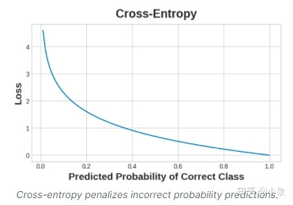
这个想法是我们希望我们的网络以 1.0 的概率预测正确的类别。预测概率离 1.0 越远，交叉熵损失就越大。我们使用交叉熵的技术原因有点微妙，但本节的主要内容就是：使用交叉熵进行分类损失；您可能关心的其他指标（如准确性）会随之提高。

Making Probabilities with the Sigmoid Function

交叉熵和准确度(accuracy)函数都需要概率作为输入，即从 0 到 1 的数字。为了将dense层产生的实值输出转换为概率，我们附加了一种新的激活函数，即 sigmoid 激活函数。

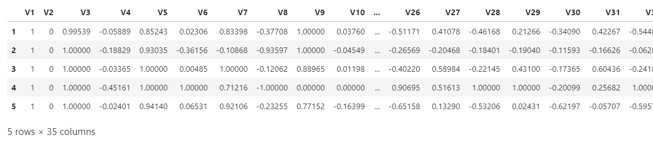
为了获得最终的预测类别，我们定义了一个阈值概率。通常是 0.5，我们将概率低于 0.5 表示标签为 0 的类，概率值为0.5 或以上表示标签为 1 的类。 threshold=0.5是 Keras 默认使用的准确度指标([accuracy metric])。一个简单的二分类例子电离层数据集([lonosphere])包含从聚焦在地球大气电离层上的雷达信号获得的特征。任务是确定信号是否显示某个物体的存在，或者只是空气。电离层数据集([lonosphere])包含从聚焦在地球大气电离层上的雷达信号获得的特征。任务是确定信号是否显示某个物体的存在，或者只是空气。

# 首先读取数据
import pandas as pd
from IPython.display import display

ion = pd.read_csv('datasets/ion.csv', index_col=0)
display(ion.head())

df = ion.copy()
df['Class'] = df['Class'].map({'good': 0, 'bad': 1})

df_train = df.sample(frac=0.7, random_state=0)
df_valid = df.drop(df_train.index)

max_ = df_train.max(axis=0)
min_ = df_train.min(axis=0)

df_train = (df_train - min_) / (max_ - min_)
df_valid = (df_valid - min_) / (max_ - min_)
df_train.dropna(axis=1, inplace=True) # drop the empty feature in column 2
df_valid.dropna(axis=1, inplace=True)

X_train = df_train.drop('Class', axis=1)
X_valid = df_valid.drop('Class', axis=1)
y_train = df_train['Class']
y_valid = df_valid['Class']

数据部分截图如下：

就像我们为回归任务所做的一样，要定义模型结构，只有一个不同的地方就是在最后一层包括一个“sigmoid”激活函数，以便模型将输出类别的概率。

from tensorflow import keras
from tensorflow.keras import layers

model = keras.Sequential([
    layers.Dense(4, activation='relu', input_shape=[33]),
    layers.Dense(4, activation='relu'),    
    layers.Dense(1, activation='sigmoid'),
])

使用其compile()方法将交叉熵损失和准确度度量添加到模型中。对于二分类问题，我们要使用“binary”版本。（多类的问题会略有不同。）Adam 优化器也适用于分类，因此我们将继续使用它。

model.compile(
    optimizer='adam',
    loss='binary_crossentropy',
    metrics=['binary_accuracy'],
)

这个特定问题中的模型可能需要相当多的 epoch 才能完成训练，因此为了方便起见，我们将包含一个提前停止回调。

early_stopping = keras.callbacks.EarlyStopping(
    patience=10,
    min_delta=0.001,
    restore_best_weights=True,
)

history = model.fit(
    X_train, y_train,
    validation_data=(X_valid, y_valid),
    batch_size=512,
    epochs=1000,
    callbacks=[early_stopping],
    verbose=0, # hide the output because we have so many epochs
)

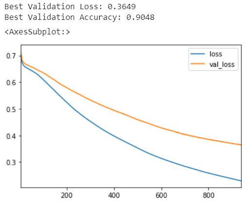
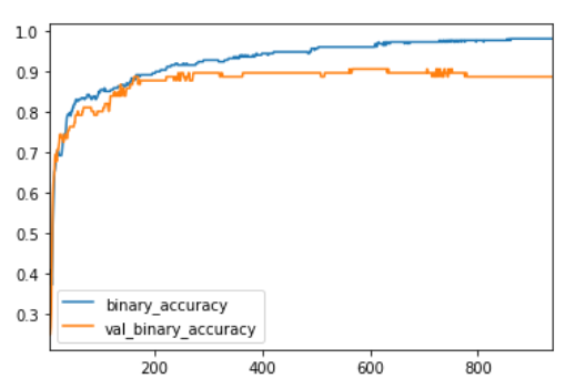
我们将一如既往地查看学习曲线，并检查我们在验证集上获得的损失和准确度的最佳值。（请记住，提前停止会将权重恢复为获得这些值的权重。）

history_df = pd.DataFrame(history.history)
# Start the plot at epoch 5
history_df.loc[5:, ['loss', 'val_loss']].plot()
history_df.loc[5:, ['binary_accuracy', 'val_binary_accuracy']].plot()

print(("Best Validation Loss: {:0.4f}" +\
      "\nBest Validation Accuracy: {:0.4f}")\
      .format(history_df['val_loss'].min(), 
              history_df['val_binary_accuracy'].max()))

练习

在本练习中，您将构建一个模型来使用二元分类器预测酒店取消。首先，加载Hotel Cancellations数据集。

import pandas as pd

from sklearn.model_selection import train_test_split
from sklearn.preprocessing import StandardScaler, OneHotEncoder
from sklearn.impute import SimpleImputer
from sklearn.pipeline import make_pipeline
from sklearn.compose import make_column_transformer

hotel = pd.read_csv('datasets/hotel.csv')

X = hotel.copy()
y = X.pop('is_canceled')

X['arrival_date_month'] = \
    X['arrival_date_month'].map(
        {'January':1, 'February': 2, 'March':3,
         'April':4, 'May':5, 'June':6, 'July':7,
         'August':8, 'September':9, 'October':10,
         'November':11, 'December':12}
    )

features_num = [
    "lead_time", "arrival_date_week_number",
    "arrival_date_day_of_month", "stays_in_weekend_nights",
    "stays_in_week_nights", "adults", "children", "babies",
    "is_repeated_guest", "previous_cancellations",
    "previous_bookings_not_canceled", "required_car_parking_spaces",
    "total_of_special_requests", "adr",
]
features_cat = [
    "hotel", "arrival_date_month", "meal",
    "market_segment", "distribution_channel",
    "reserved_room_type", "deposit_type", "customer_type",
]

transformer_num = make_pipeline(
    SimpleImputer(strategy="constant"), # there are a few missing values
    StandardScaler(),
)
transformer_cat = make_pipeline(
    SimpleImputer(strategy="constant", fill_value="NA"),
    OneHotEncoder(handle_unknown='ignore'),
)

preprocessor = make_column_transformer(
    (transformer_num, features_num),
    (transformer_cat, features_cat),
)

# stratify - make sure classes are evenlly represented across splits
X_train, X_valid, y_train, y_valid = \
    train_test_split(X, y, stratify=y, train_size=0.75)

X_train = preprocessor.fit_transform(X_train)
X_valid = preprocessor.transform(X_valid)

input_shape = [X_train.shape[1]]

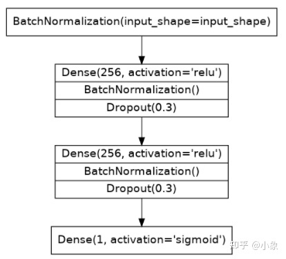
我们这次将使用一个同时具有批量归一化和 dropout 层的模型。使用下图给出的架构定义模型：

from tensorflow import keras
from tensorflow.keras import layers

# YOUR CODE HERE: define the model given in the diagram
model = keras.Sequential([
    layers.BatchNormalization(input_shape=input_shape),
    layers.Dense(256, activation='relu'),
    layers.BatchNormalization(),
    layers.Dropout(rate=0.3),
    layers.Dense(256, activation='relu'),
    layers.BatchNormalization(),
    layers.Dropout(rate=0.3),
    layers.Dense(1, activation='sigmoid'),
])

现在使用 Adam 优化器和交叉熵损失和准确度度量的二进制版本编译模型。

model.compile(
    optimizer='adam',
    loss='binary_crossentropy',
    metrics=['binary_accuracy'],
)

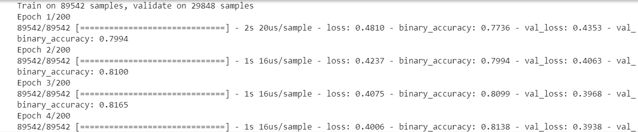
最后，运行此单元来训练模型并查看学习曲线。它可能会运行大约 60 到 70 个 epoch，这可能需要一两分钟。

early_stopping = keras.callbacks.EarlyStopping(
    patience=5,
    min_delta=0.001,
    restore_best_weights=True,
)
history = model.fit(
    X_train, y_train,
    validation_data=(X_valid, y_valid),
    batch_size=512,
    epochs=200,
    callbacks=[early_stopping],
)

history_df = pd.DataFrame(history.history)
history_df.loc[:, ['loss', 'val_loss']].plot(title="Cross-entropy")
history_df.loc[:, ['binary_accuracy', 'val_binary_accuracy']].plot(title="Accuracy")

运行后的部分截图如下：

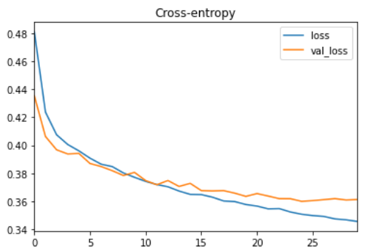
您如何看待学习曲线？它看起来像模型欠拟合还是过拟合？cross-entropy是accuracy的一个很好的替代品吗？虽然我们可以看到训练损失继续下降，但提前停止回调防止了任何过度拟合。此外，准确度上升的速度与交叉熵下降的速度相同，因此最小化交叉熵似乎是一个很好的替代方案。总而言之，这次训练看起来很成功

AIStation

AI站长的个人学习笔记

深度学习入门六----分类问题

Binary Classification

Accuracy and Cross-Entropy

Making Probabilities with the Sigmoid Function

练习

您还没有登录，请您登录后发表评论。